
By José Carlos Gonzáles Tanaka
On this weblog, I wish to current one of many superior information evaluation strategies accessible in Python to the quant buying and selling neighborhood to help their analysis ambitions. It has been completed in a easy and hands-on method. You will discover the TGAN code on GitHub as nicely.
Why TGAN?
You’ll encounter conditions the place each day monetary information is inadequate to backtest a technique. Nonetheless, artificial information, following the identical actual information distribution, may be extraordinarily helpful to backtest a technique with a ample variety of observations. The Generative adversarial community, a.okay.a GAN, will assist us generate artificial information. Particularly, we’ll use the GAN mannequin for time collection information.
Weblog Targets & Contents
On this weblog, you’ll be taught:
- The GAN algorithm definition and the way it works
- The PAR synthetizer to make use of the time-series GAN (TGAN) algorithm
- Methods to backtest a technique utilizing artificial information created with the TGAN algorithm
- The advantages and challenges of the TGAN algorithm
- Some notes to take note of to enhance the outcomes
This weblog covers:
Who is that this weblog for? What must you already know?
For any dealer who would possibly take care of scarce monetary information for use to backtest a technique. It’s best to already know the right way to backtest a technique, about technical indicators, machine studying, random forest, Python, deep studying.
You may find out about backtesting right here:
To find out about machine studying associated subjects observe the hyperlinks right here:
If you wish to know extra about producing artificial information, you may test this text on Forbes.
What the GAN algorithm is, and the way it works
A generative adversarial community (GAN) is a sophisticated deep studying structure that consists of two neural networks engaged in a aggressive coaching course of. This framework goals to generate more and more practical information based mostly on a chosen coaching dataset.
A generative adversarial community (GAN) consists of two interconnected deep neural networks: the generator and the discriminator. These networks operate inside a aggressive surroundings, the place the generator’s aim is to create new information, and the discriminator’s position is to find out whether or not the produced output is genuine or artificially generated.
From a technical perspective, the operation of a GAN may be summarized as follows. Whereas a fancy mathematical framework underpins the whole computational mechanism, a simplified rationalization is introduced beneath:
The generator neural community scrutinizes the coaching dataset to establish its underlying traits. Concurrently, the discriminator neural community analyzes the unique coaching information, independently recognizing its options.
The generator then alters particular information attributes by introducing noise or random modifications. This modified information is subsequently introduced to the discriminator.
The discriminator assesses the probability that the generated output originates from the real dataset. It then gives suggestions to the generator, advising it to attenuate the randomness of the noise vector in subsequent iterations.
The generator seeks to reinforce the possibilities of the discriminator making an misguided judgment, whereas the discriminator strives to scale back its error fee. By way of iterative coaching cycles, each the generator and discriminator progressively develop and problem each other till they obtain a state of equilibrium. At this juncture, the discriminator is unable to tell apart between actual and generated information, signifying the conclusion of the coaching course of.
On this case, we’ll use the SDV library the place we now have a particular GAN algorithm for time collection. The algorithm follows the identical process from above, however on this time-series case, the discriminator learns to make an identical time collection from the actual information by making a match between the actual and artificial returns distribution.
The PAR synthesizer from the SDV library
The GAN algorithm mentioned on this weblog comes from the analysis paper on “Sequential Fashions within the Artificial Information Vault“ by Zhang printed in 2022. The precise title of the algorithm is the conditional probabilistic auto-regressive (CPAR) mannequin.
The mannequin makes use of solely multi-sequence information tables, i.e. multivariate time collection information. The excellence right here is that for every asset value, you’ll want a context variable that may establish the asset all through the estimation and that doesn’t fluctuate inside the sequence datetime index or rows, i.e., these context variables don’t change over the course of the sequence. That is known as “contextual data”. Within the inventory market, the business, and the agency sector denote the asset “context”, i.e., the context that the asset belongs to.
Some issues to notice about this algorithm are:
- A various vary of information varieties is offered, together with numeric, categorical, datetime, and others, in addition to some lacking values.
- A number of sequences may be integrated inside a single dataframe, and every asset can have a unique variety of observations.
- Every sequence has its personal distinct context.
- You’re not in a position to run this mannequin with a single asset value information. You’ll really need multiple asset value information.
Backtest a machine-learning-based technique utilizing artificial information
Let’s dive rapidly into our script!
First, let’s import the libraries
Let’s import the Apple and Microsoft inventory value information from 1990 to Dec-2024. We obtain the two inventory value information individually after which create a brand new column named “inventory” that may have for all rows the title of every inventory comparable to its value information. Lastly, we concatenate the information.
Let’s create a operate to create artificial datetime indexes for our new artificial information:
Let’s now create a operate that will likely be used to create the artificial information. The operate rationalization goes in steps like these:
- Copy the actual historic dataframe
- Create the artificial dataframe
- Create a context column copying the inventory column.
- We’ll set the metadata construction. This construction is important for the GAN algorithm on the SDV library:
- Right here we outline the column information sort collectively. We specify the inventory column as ID, as a result of this may establish the time collection that belong to every inventory.
- We specify the sequence index, which is simply the Date column describing the time collection datetime indexes for every inventory value information.
- We set the context column to match the inventory column, which serves as a ‘trick’ to affiliate the Quantity and Returns columns with the identical asset value information. This strategy ensures that the synthesizer generates fully new sequences that observe the construction of the unique dataset. Every generated sequence represents a brand new hypothetical asset, reflecting the overarching patterns within the information, however with out comparable to any real-world firm (e.g., Apple or Microsoft). Through the use of the inventory column because the context column, we keep consistency within the asset value return distribution.
- We set the ParSynthetizer mannequin object. In case you will have an Nvidia GPU, please set cuda to True, in any other case, to False.
- Match the GAN mannequin for the Quantity and value return information. We don’t enter OHL information as a result of the mannequin would possibly receive Excessive costs beneath the Low information, or Low costs greater than the Excessive costs, and so forth.
- Right here we output the artificial information based mostly on a definite seed. For every seed:
- We specify a personalized state of affairs context, the place we outline the inventory and context as equal so we get the identical Apple and Microsoft value return distribution.
- Get the Apple and Microsoft artificial pattern utilizing a selected variety of observations named as sample_num_obs
- Then we save solely the “Image” dataframe in synthetic_sample
- Compute the Shut costs
- Get the historic imply return and commonplace deviation for the Excessive and Low costs with respect to the Shut costs.
- Compute the Excessive and Low costs based mostly on the above.
- Create the Open costs with the earlier Shut costs.
- Spherical the costs to 2 decimals.
- Save the artificial information right into a dictionary relying on the seed quantity. The seed dialogue will likely be completed later.
The next operate is similar described in my earlier article on Danger Constrained Kelly Criterion.
The next operate is about utilizing a concatenated pattern (with actual and artificial information) and:
And this final operate is about getting the enter options and prediction characteristic individually for the practice and take a look at pattern.
Subsequent:
- Set the random seed for the entire script
- Specify 4 years of information for becoming the artificial mannequin and the machine-learning mannequin
- Set the variety of observations for use to create the artificial information. Put it aside as test_span
- Set the preliminary yr for the backtesting yr durations.
- Get the month-to-month indexes and the seeds checklist defined later.
We create a for-loop to backtest the technique:
- The for loop goes via every month of the 2024 yr.
- It’s a walk-forward optimization the place we optimize the ML mannequin parameter on the finish of every month and commerce the next month.
- For every month, we estimate 20 random-forest algorithms. Every mannequin will likely be completely different as per its random seed. For every mannequin, we create artificial information for use for the actual ML mannequin.
The for loop steps go like this:
- Specify the present and subsequent month finish.
- Outline the span between the present and month finish datetimes
- We outline the information pattern as much as the subsequent month and use the final 1000 observations plus the span outlined above.
- Outline 2 dictionaries to save lots of the accuracy scores and the fashions.
- Outline the information pattern for use to coach the GAN algorithm and the ML mannequin. Put it aside within the tgan_train_data variable.
- Create the artificial information for every seed utilizing our earlier operate named “create_synthetic_data”. Select the Apple inventory solely for use to backtest the technique.
- For every seed
- Create a brand new variable to save lots of the corresponding artificial information as per the seed.
- Replace the Open first value remark.
- Concatenate the actual Apple inventory value information with its artificial information.
- Sor the index
- Create the enter options
- Break up the information into practice and take a look at dataframes.
- Separate the enter and prediction options from the above 2 dataframes as X and y.
- Set the random-forest algo object
- Match the mannequin with the practice information.
- Save the accuracy rating utilizing the take a look at information.
- Get the most effective mannequin seed as soon as we estimate all of the ML fashions. We choose the most effective random forest mannequin based mostly on the artificial information predictions utilizing the accuracy rating.
- Create the enter options
- Break up the information into practice and take a look at dataframes.
- Get the sign predictions for the subsequent month.
- Proceed the loop iteration
The next technique efficiency computation, plotting and pyfolio-based efficiency tear sheet relies on the identical article referenced earlier on risk-constrained Kelly Criterion.
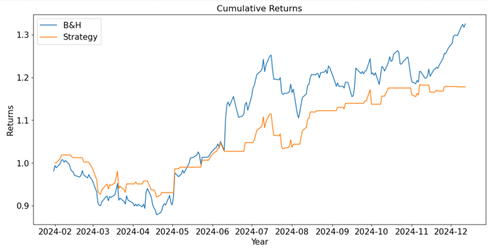
From the above pyfolio outcomes, we’ll create a abstract desk:
Metric | B&H Technique | ML Technique |
Annual return | 41.40% | 20.82% |
Cumulative returns | 35.13% | 17.78% |
Annual volatility | 22.75% | 14.99% |
Sharpe ratio | 1.64 | 1.34 |
Calmar ratio | 3.24 | 2.15 |
Max Drawdown | 12.78% | 9.69% |
Sortino ratio | 2.57 | 2.00 |
We are able to see that, general, we get higher outcomes utilizing the Purchase-and-Maintain technique. Regardless that the annual return is greater for the B&H technique, the volatility is decrease for the ML technique utilizing the artificial information for backtesting; though the B&H technique has the next Sharpe ratio. The Calmar and Sortino ratios are greater for the B&H technique, though we receive a decrease max drawdown with the ML technique.
The advantages and challenges of the TGAN algorithm
The advantages:
- You may cut back information assortment prices as a result of artificial information may be created based mostly on a decrease variety of observations in comparison with having the entire information of a selected asset or group of property. This enables us not to focus on information gathering however on modeling.
- Larger management of information high quality. Historic information is just a single path of the whole information distribution. Artificial information with good high quality can provide you a number of paths of the identical information distribution, permitting you to suit the mannequin based mostly on a number of eventualities.
- Because of the above, the mannequin becoming on artificial information will likely be higher, and the ML fashions may have better-optimized parameters.
The challenges:
- The TGAN algorithm becoming can take a very long time. The larger the information pattern to coach the TGAN, the longer it would take to suit the information. When coping with thousands and thousands of observations to suit the algorithm, you’ll face a very long time to get it accomplished.
- Resulting from the truth that the generator and discriminator networks are adversarial, GANs often expertise coaching instability, i.e., the mannequin doesn’t match the information. To make sure steady convergence, hyperparameters have to be fastidiously adjusted.
- TGAN can are inclined to mannequin collapse: If there’s an imbalance coaching between the mannequin’s generator and discriminator, there’s a decreased variety of samples generated for artificial information. Hyperparameters, as soon as once more, ought to be adjusted to take care of this problem.
Some notes concerning the TGAN-based backtesting mannequin
Please discover beneath some issues to enhance within the script
- You may enhance the fairness curve by making use of threat administration thresholds corresponding to stop-loss and take-profit targets.
- We have now used the accuracy rating to decide on the most effective mannequin. You can have used some other metric such because the F1-score, the AUC-ROC, or technique efficiency metrics corresponding to annual return, Sharpe ratio, and so forth.
- For every random forest, you can have obtained multiple time collection (sequence) for every asset to backtest a technique for a number of paths (sequences). We did this arbitrarily to scale back the time spent on operating the algorithm each day and for demonstration functions. Creating a number of paths to backtest a technique would give your finest mannequin a extra sturdy technique efficiency. That’s one of the best ways to revenue from artificial information.
- We compute the enter options for the actual inventory value a number of instances after we can really do it as soon as. You may tweak the information to just do that.
- The ParSynthetizer object outlined in our operate referred to as “create_synthetic_data” has an enter referred to as “epochs”. This variable permits us to cross the whole coaching dataset into the TGAN algorithm (utilizing the generator and discriminator). We have now used the default worth which is 128. The upper the variety of epochs, the upper the standard of your artificial pattern. Nonetheless, please take note of that the upper the epoch quantity, the longer the time spent for the GAN mannequin to suit the information. It’s best to steadiness each as per your compute capability and optimization finest time on your walk-forward optimization course of.
- As an alternative of making the proportion returns for the non-stationary options, you can have used the ARFIMA mannequin utilized to every non-stationary characteristic and use the residuals because the enter characteristic. Why? Verify our ARFIMA mannequin weblog article.
- Don’t neglect to make use of transaction prices to simulate higher the fairness curve efficiency.
Conclusion
The aim of this weblog was to:
– Current you with the TGAN algorithm to analysis additional.
– Present a backtesting code script that may be readily tweaked.
– Focus on the advantages and shortcomings of utilizing TGAN algorithm in buying and selling.
– Recommend subsequent steps to proceed working.
To summarize, we utilized a number of random forest algorithms every day and chosen the most effective one based mostly on the most effective Sharpe ratio obtained with the test-data created utilizing artificial information.
On this case, we used a time-series-based GAN algorithm. Watch out about this, there are numerous GAN algorithms however few for time-series information. It’s best to use the latter mannequin.
In case you are fascinated about superior algorithmic buying and selling methods, we suggest you the next programs
- Govt Programme in Algorithmic Buying and selling: First step to construct your profession in Algorithmic buying and selling.
- AI in Buying and selling Superior: Self-paced programs centered on Python.
File within the obtain:
- The Python code snippets for implementing the technique are offered, together with the set up of libraries, information obtain, create related capabilities for the backtesting loop, the backtesting loop and efficiency evaluation.
All investments and buying and selling within the inventory market contain threat. Any resolution to put trades within the monetary markets, together with buying and selling in inventory or choices or different monetary devices is a private resolution that ought to solely be made after thorough analysis, together with a private threat and monetary evaluation and the engagement {of professional} help to the extent you imagine mandatory. The buying and selling methods or associated data talked about on this article is for informational functions solely.


