Calculation, Covariance Matrix, and Python Examples

By Tsotne Kutalia

How would you measure the chance of holding a single asset like an organization inventory? How would you evaluate two property when it comes to their dangers? How would you choose an asset to be added to your present portfolio?

Earlier than Nineteen Fifties, buyers would search solutions in monetary studies reminiscent of stability sheet or revenue assertion and get some qualitative perceptions concerning the efficiency of a given asset. In any other case, they’d learn information associated to a specific asset and brainstorm concerning the probability of the worth rise or fall.

Then got here Harry Markowitz, a younger PhD pupil in Chicago College and wrote a thesis named “Portfolio Choice” later famously named “Fashionable Portfolio Idea” or just MPT. He instructed buyers to look at the relationships between the anticipated return () and customary deviation () of returns. This was a milestone on the earth of investments and gave delivery to quantitative finance as a self-discipline.

This weblog is self-sufficient within the sense that we’ll construct the subject from the bottom up. The next sections are lined.

Conditions:

1. Random Variable
2. Normal Deviation
3. Covariance
4. Normal Regular Distribution
5. Introduction to portfolio administration

Perceive the return of a single asset

What’s return on an asset?

Suppose that at a given second an asset is price $100 and you purchase it. Subsequent second (say in a single week) the worth rises to $110. The return in your funding then is

In different phrases, by holding this asset, you’d acquire 10% in your funding. Typically talking, the return on an asset in a single interval is computed by the components

Since it’s unknown what worth ( R_t ) will take, we regard it as a random variable. For simplicity, we will confer with a random variable as a variable whose worth is unknown upfront.

Instance 1.1:

The instance consists of the Exon Mobil Corp. (XOM) inventory costs. The returns are computed in keeping with (1.1.1) in excel. The final column (D) comprises the components for the column C. The primary column comprises the dates sorted in descending order in format MM/DD/YYYY. So the month-to-month returns are supplied.

The identical computations will be carried out in python as follows:

Estimating variance and customary deviation as threat measures

From the realizations of returns (i.e. noticed historic worth of return – the random variable R), it’s attainable to estimate the anticipated return of a given asset. Assuming equal weights for every realization of return, the anticipated return, denoted by R is given by

This imply worth of returns is one attribute of numerical knowledge measuring the central tendency of the information. The estimated variance of the random variable R alternatively, measures the variability of the information across the imply is given by the next components

The variance of returns, as proven in (1.2.2) is the common squared deviation from the anticipated return. It measures how a lot risky the inventory returns are with respect to the imply. Thus, the variance is taken because the measure of threat of an asset. In different phrases, the chance is the common squared deviation from the anticipated returns.

Nonetheless, the squared distinction between the person asset returns and the imply has no any significant interpretation. With a view to convey the amount again into the unique items, we compute the sq. root of the variance to acquire the usual deviation of returns

Normal deviation is a threat measure. Decrease the worth of s, much less dangerous a given asset is taken into account to be and vise versa.

Instance 2.1

The anticipated day by day return of the inventory occurs to be round 1.35% computed by (1.2.1).  Now we measure by how a lot the person returns are scattered round this worth on common. In response to (1.2.2)

And the corresponding customary deviation computed by (1.2.3) is s = √s² = 0.00385.

The identical portions will be computed in python with the next easy fragment of the code:

In consequence, we receive σ² = 0.00148 and σ = 0.038473 as month-to-month variance and customary deviation respectively.

Perceive relationships between two property

Covariance coefficient

Up to now, we mentioned the anticipated return and customary deviation of a single random variable. Now contemplate two random variables, X and Y, noticed as pairs (x₁, y₁), (x₂, y₂), …, (x_n, y_n). So the pattern measurement is n, i.e. we have now n pairs. The covariance coefficient between two random variables measures their linear dependence and is computed by

If s_xy > 0, the 2 variables are positively associated, i.e. they transfer in the identical route. Merely put, growing the worth of X is adopted by a rise in Y and vice versa – reducing the worth of X causes the worth of Y to drop. Suppose X is an actual property space measured in sq. toes and Y is the corresponding worth measured in hundreds of {dollars}. Then it’s anticipated that the covariance between these variables will probably be constructive, implying that bigger actual property prices extra and smaller one is price much less.

So long as s_xy < 0, the 2 variables are negatively associated, i.e. they transfer in the other way. Merely put, growing the worth of X is adopted by a lower in Y and vice versa – reducing the worth of X causes the worth of Y to rise. Suppose X is a worth of a sure product measured in {dollars} and Y is the corresponding demand measured in items offered. Then it’s anticipated that the covariance between these variables will probably be detrimental, implying that larger worth ends in decrease demand and cheaper price ends in larger demand.

s_xy = 0 expresses the statistical independence of X and Y. In different phrases, altering the worth of X has no impact on the worth of Y.

Having mentioned the covariance coefficient for 2 summary random variables X and Y for simplicity, we now repeat the identical components for the random variables which signify the returns of two property in a given portfolio: R₁ and R₂, i.e. contemplate a portfolio of two property with respective returns R₁ and R₂. Then the pattern covariance coefficient computed based mostly on the realizations is equivalent to (2.1.1 a)

We might interpret the constructive and detrimental (and nil) covariances equally to X and Y. Consider the case s_R1R2 > 0 as if the property (like shares) are chosen from the identical business. Thus, related elements have an effect on each. So, growing the worth of 1 inventory, trigger the worth of one other to rise. The instance of this case could be two shares from tech business, or each shares from car business, and many others. Reverse holds true for s_R1R2 < 0. Particularly, on this case, growing the worth of 1 inventory ends in a fall of one other. You’ll be able to consider this case as if the shares have been chosen for complement industries like airways and oil manufacturing. The next instance illustrates the case.

Instance cont’d:

Contemplate a portfolio consisting of two property. Exon Mobil Corp. (XOM) and American Airways Group Inc. (AAL) shares. These corporations are from negatively associated industries. In different phrases, American Airlies Inc. is determined by the oil worth. Greater the oil worth (i.e. larger the XOM worth ) decrease the AAL worth is and vice versa. In different phrases, airways and oil producing industries transfer in reverse instructions. Their month-to-month costs for the final 12 months are given beneath

Allow us to denote their returns by R₁ and R₂, respectively. Computations of returns are carried out by (1.1.1) and we receive

With a view to compute the covariance coefficient, one must first derive
R₁ and
R₂.

and by (2.1.1 b) the covariance is computed as

In excel, that is achieved by a single perform

In consequence, we receive s=-0.00066, a detrimental worth. Allow us to take into consideration this for a second. American Airways (AAL) is a shopper of oil as vitality. If the oil worth rises, benefiting Exon Mobil (XOM), the AAL worth drops. The alternative occurs when the oil worth drops. So, we will conclude that AAL and XOM transfer in reverse instructions.

Variance and customary deviation of a portfolio with two property

Suppose we have now a portfolio consisting of two property with the corresponding returns R₁ and R₂. Let the weights vector be w = [w₁, w₂]. The variance of such portfolio is computed by

Right here the final time period makes a giant distinction. What we see is that the portfolio variance isn’t just the weighted sum of two variances, however it additionally has the third phrases which comprises the covariance coefficient. That is essential.

Suppose you handle to seek out two property with the identical anticipated return and detrimental covariance between the returns. As an alternative of placing all of your funding into one of many property, you might cut up it into these two property, and whilst you preserve the identical anticipated return, the detrimental final time period of (2.2.1) would make your total threat decrease. From (2.2.1), we will derive the usual deviation of the portfolio as

Observe that in (2.2.1), if s_xy=0 i.e. you discover unbiased property), then the portfolio variance will simply be the weighted sum of two variances

Allow us to now outline the covariance matrix as follows

the place the weather of the matrix signify the covariances measured between all pairs of particular person returns.

Now allow us to contemplate the covariance coefficient by (2.1.1 b). If we compute the covariance of a random variable X with respect to itself, we might receive

So, that is basically the variance of R₁ computed by (1.2.2) and thus, (2.2.3 a) turns into

and therefore, it’s referred to as the variance-covariance matrix. On the diagonal, you discover the variances of the random variables.

So long as we have now the definition of the covariance matrix and the weights vector, we will rewrite (2.2.1) when it comes to matrices as follows

Out of which the portfolio customary deviation will be computed by merely taking the sq. root. Extra fully outlined, the portfolio customary deviation is

Instance cont’d:

Suppose we put equal weights into the portfolio w = [w₁, w₂] = [0.5 0.5]. The variance-covariance matrix then is

Then by (2.2.4) the variance of the portfolio returns turns into

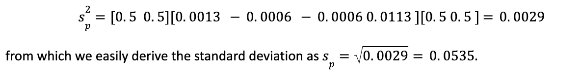
In Excel, the computations are illustrated beneath

The identical computations will be carried out by way of python as illustrated beneath

Perceive multi asset portfolio

Variance-covariance matrix for a multi – asset portfolio

Suppose we have now a portfolio of N property, if we compute the covariance phrases between all of the pairs, s_RiRj

then we will generalize the variance-covariance matrix in (2.2.3 b) right into a kind

during which the squared phrases on the diagonal confer with the variances of every asset returns (i.e. of R₁, R₂, …, R_N). All phrases generally are computed by the components (2.1.1 b).

Instance Cont’d:

We proceed to assemble the covariance matrix for a portfolio consisting of greater than 2 property. First, we add one other inventory – Amazon.com Inc. (AMZN) to the prevailing portfolio. So, it now turns into N=3 asset portfolio. The returns for all shares are computed by (1.1.1) in keeping with the strategy we mentioned above. Then the covariance matrix components will be computed by (2.1.1 b). In excel that is achieved by covariance perform of Knowledge Evaluation bundle in Knowledge tab.

The ensuing covariance matrix is given beneath

The identical matrix will be constructed by way of python as follows

Variance and customary deviation of a portfolio of multi  – property

On this part, we generalize the dialogue of part 2.2. Now suppose we have now a multi-asset portfolio with weights vector w = [w₁ w₂ … w_N]. Then the variance of the portfolio will be written as

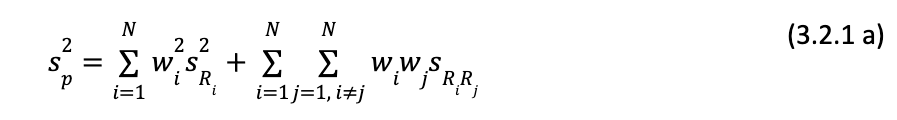
which is actually (2.2.1) generalized. We will rewrite this components right into a matrix kind

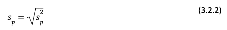
out of which we derive the usual deviation as

Exaple Cont’d:

Suppose we cut up the funding into the weights w = [w₁ w₂ w₃] = [0.4 0.3 0.3]. The computations based mostly on (3.2.1 b) is illustrated beneath

Python analogue for computation of variance and customary deviation is given beneath

Threat of an asset or a portfolio is measured by the variance and customary deviation of its return. They measure by how a lot on common the returns deviate from the imply worth. Greater (decrease) the variance or customary deviation, larger (decrease) the chance is.

Covariance coefficient measures the dependence between two asset returns. Whether it is constructive (detrimental), growing the return of one in every of them, causes one other to additionally enhance (lower) and whether it is detrimental, then growing the return of one in every of them, causes one other to lower (enhance). It’s a good suggestion to hunt property with detrimental covariance, since this may scale back total threat of a portfolio. That is referred to as the diversification impact.

So long as covariances between every pair within the portfolio is thought (or at the very least estimated), it’s attainable to compute the chance of the complete portfolio utilizing the variance/covariance matrix examined above.

Information within the obtain:

The Excel file illustrates development of portfolio variance-covariance matrix step-by-step. There you’ll find an instance of a portfolio consisting of two and three property individually.

The Python code snippet illustrates the development of a variance-covariance matrix for a portfolio consisting of three property. The code file can be utilized as a template with slight modifications.

Login to Obtain

Bibliography:

Bodie Z.,  Kane A.,  Marcus A.J., (2008) Investments. The McGraw-Hill/Irwin collection in finance, insurance coverage and actual property)

Additional Studying:

1. Portfolio Optimization Strategies
2. Fashionable Portfolio Administration Utilizing Capital Asset Pricing Mannequin and Fama-French Three Issue Mannequin
3. Portfolio Optimization Utilizing Monte Carlo Simulation
4. Portfolio Evaluation – Efficiency Measurement and Analysis

All investments and buying and selling within the inventory market contain threat. Any determination to position trades within the monetary markets, together with buying and selling in inventory or choices or different monetary devices is a private determination that ought to solely be made after thorough analysis, together with a private threat and monetary evaluation and the engagement {of professional} help to the extent you imagine crucial. The buying and selling methods or associated data talked about on this article is for informational functions solely.