
By Tostne Kutalia
If you’re studying this weblog, which means that you might be conscious of Worth at Threat, or just VaR which is the most important loss that may be incurred by a portfolio with a given confidence degree (i.e. a pre-specified chance degree).
Nonetheless, there’s a vital downside which the VaR as a threat measure carries. Particularly, it tells us the brink of potential loss however not how unhealthy the loss will be past that threshold.
For instance, if a portfolio’s 1-day VaR is $1 million at a 95% confidence degree, you don’t know the way a lot the loss might be within the remaining 5% of the instances. As well as, it doesn’t account for “tail threat” or excessive occasions which will result in bigger losses. This brings us to one more statistical threat measure referred to as Anticipated Shortfall (ES), which fixes this drawback to some extent.
As seen within the previous paragraph, to be totally outfitted to know the subject of Anticipated Shortfall, first one must have the information of VaR. What follows is the checklist of conditions wanted alongside their descriptions.
Conditions
- The introduction to VaR is defined right here. By studying the referred weblog, you’ll discover ways to compute and interpret portfolio VaR, its limitations and benefits in easiest and shortest attainable approach.
- To get a complete information about VaR and associated subjects, you possibly can discuss with the weblog “Worth at Threat”. Right here you will see that an in depth clarification of VaR, its computation in varied methods. As well as, this weblog offers a protection of subjects like Marginal VaR, Incremental VaR and Element VaR. In brief, these VaR instruments measure the consequences of adjusting portfolio positions on present portfolio VaR.
What’s Anticipated Shortfall (ES)
Merely put, Anticipated Shortfall is the common loss past VaR. It measures the anticipated loss within the tail of a distribution past a sure quantile degree (e.g., 95%). It offers perception into the potential losses exceeding the Worth at Threat (VaR). Clearly, we specify the arrogance degree by which ES is computed. Beneath is the geometric illustration of ES alongside with VaR. Listed here are the steps for the computation of ES:
1. Outline Parameters
- Confidence Stage (c): Select the arrogance degree, usually 95% or 99%.
- Loss Distribution: Have the historic or simulated distribution of portfolio returns or losses.
- Calculate portfolio worth in danger (( textual content{VaR}_p )): That is additionally computed by the identical confidence degree.

the place z stands for traditional regular quantile similar to c chance, p is the usual deviation of portfolio returns and W represents the portfolio worth in {dollars}.
2. Calculate Anticipated Loss Past (VaR): That is in impact the Anticipated Shortfall and is computed by the components

the place ( L ) denotes the loss as a random variable (i.e. the attainable worth of precise loss). The above components is learn because the anticipated (common) loss on condition that this loss is larger than ( textual content{VaR}_{p} ).
The components of Anticipated Shortfall is a theoretical one. We take empirical (historic knowledge primarily based) and analytic approaches to compute this amount.
Empirical Strategy:
The only strategy to compute the ES from historic knowledge is to search out VaR utilizing the non-parametric methodology. So long as VaR is computed, one wants to easily common out all traditionally noticed values past this amount.
Instance:
We prolong the instance given within the part “Non-Parametric VaR” of weblog Worth at Threat. Particularly, so long as the annual VaR (on this case we use VaR (zero), nevertheless VaR (imply) would additionally work) has been computed, we compute the common worth of losses past this degree. Notice that these portions are computed within the weblog on the given hyperlink above. See the connected Excel file for full computations as effectively.
The given portfolio on this instance is initially value $1,000,000 and it consists of three property. First, the portfolio values are computed.
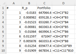
Then we compute the loss incurred in comparison with the preliminary worth of the portfolio.
The VaR seems to be $326,554.42 (computed within the weblog above) whereas the Anticipated Shortfall is $337,559.84. This amount is computed by (2) as illustrated beneath
We interpret this amount because the anticipated loss in excessive circumstances. To make it clearer and less complicated, $337,559.84 is the anticipated quantity if the precise loss surpasses $326,554.42 (the VaR). It is a self-explanatory quantity within the sense that it offers an impression about what to anticipate in excessive instances, i.e. if the 5% chance of loss exceeding VaR is realised.
Analytic Strategy:
As a substitute of computing ES by non-parametric methodology, so long as the parameters of loss distribution are estimated, we will compute it by way of the analytic methodology. Particularly, the ES given by (2) is equal to

the place ( l ) denotes the loss. So this components simply offers the common of the losses past ( textual content{VaR}_{p} ) adjusted to the arrogance degree ( c ). If the distribution is understood, the computation turns into less complicated. Within the easiest case, assuming the losses are usually distributed (which is sort of a primary assumption, not essentially true although), we compute the ES by the next components:

the place L and L denote the imply and normal deviation of losses respectively. Notice that these portions have the indexes to distinguish them from portfolio return imply and normal deviation. z often represents the usual regular quantile similar to c confidence degree and is the usual regular density operate. (Could be nice to have a hyperlink for chance distributions). The computations are given within the instance beneath
Instance cont’d:
Now we compute the ES utilizing the analytic, a.okay.a. parametric methodology. Estimated imply and normal deviations are respectively.

we will compute ES by (4) to be $328,130.07.
Notice that this amount is barely decrease than the ES worth computed by non-parametric methodology, nevertheless each definitely are larger than VaR.
Professionals of utilizing Anticipated Shortfall as a threat measure:
1. Accounts for Tail Threat
- Not like Worth at Threat (VaR), which solely considers the brink loss at a given confidence degree, ES averages all losses past the VaR, offering a extra complete view of tail threat.
2. Higher threat sensitivity
- Not like Worth at Threat (VaR), which solely considers the brink loss at a given confidence degree, ES averages all losses past the VaR, offering a extra complete view of tail threat.
3. Regulatory Acceptance
- ES is more and more utilized in monetary laws (e.g., Basel III) as a result of it overcomes a few of VaR’s limitations, equivalent to ignoring losses past the VaR threshold.
4. Flexibility
- ES will be utilized to numerous distributions and threat eventualities, together with heavy-tailed distributions and non-normal knowledge.
Cons and Limitations of utilizing Anticipated Shortfall as a threat measure:
1. Estimation challenges
- ES requires correct modeling of the tail of the loss distribution, which is tough in apply because of the shortage of utmost loss knowledge.
2. Knowledge and dependence
- Historic and simulation-based strategies can produce inaccurate ES estimates if the information doesn’t adequately seize future threat eventualities.
3. Computational depth
- Calculating ES will be computationally demanding, particularly for advanced portfolios or when utilizing Monte Carlo simulation.
4. Interpretation complexity
- The selection of the arrogance degree (c) considerably impacts ES, introducing a level of subjectivity.
5. Sensitivity to mannequin assumptions
- The accuracy of ES relies upon closely on the assumed distribution of losses. Mis-specification of the distribution can result in unreliable estimates.
Conclusion
This weblog coated an attention-grabbing amount – Anticipated Shortfall (ES). ES is the anticipated loss surpassing the VaR degree. It offers a priceless data within the sense that throughout the realization of utmost losses, one is aware of what to anticipate on common. VaR as a threat measure, fails to account for this loss. There are a number of methods to compute Anticipated Shortfall. Examples got illustrating computations of ES by non-parametric methodology, which provides an estimate utilizing the historic knowledge and an analytic methodology, which is extra sturdy assuming the distribution of losses is understood and the parameters of the distribution (like imply and normal deviation) estimated. Lastly, the subject is summarized by offering the checklist of professionals and cons of utilizing ES as a threat measure.
Recordsdata within the obtain:
The excel file illustrates the computation of Anticipated Shortfall for a portfolio consisting of three shares. Portfolio VaR is computed first. The Anticipated Shortfall is computed by parametric and non-parametric approaches.
The python code snippets illustrate the computation of Anticipated Shortfall step-by-step. The portfolio VaR is computed first on high of which the portfolio Anticipated Shortfall is calculated.
Bibliography:
- Jorion, P. (2001). Worth At Threat: The brand new benchmark for managing Monetary threat. New York: McGraw Hill.
All investments and buying and selling within the inventory market contain threat. Any determination to put trades within the monetary markets, together with buying and selling in inventory or choices or different monetary devices is a private determination that ought to solely be made after thorough analysis, together with a private threat and monetary evaluation and the engagement {of professional} help to the extent you consider needed. The buying and selling methods or associated data talked about on this article is for informational functions solely.


