
By Tostne Kutalia
What’s the largest quantity I’d lose on an funding? That is the query each investor asks in some unspecified time in the future in time. In different phrases, given the pre specified stage of certainty (i.e. chance), an investor desires to be assured that the funding loss doesn’t surpass a sure stage. Worth at Threat (VaR) is a statistical measure of largest potential loss (akin to a sure confidence stage) which addresses this downside. The primary benefit of VaR is that it summarizes threat in a single, easy-to-understand quantity.
Stipulations:
- You’ve learn (my different weblog: https://weblog.quantinsti.com/value-at-risk/)
- You’ve the essential data of chance distributions.
On this weblog we are going to look at the next subjects:
- What’s VaR and why use it as a threat measure?
- Non-parametric/parametric VaR as a statistical measure
- Non-parametric VaR
- Parametric VaR
- Portfolio VaR and predominant VaR instruments. Definitions and interpretations.
- Portfolio VaR
- Marginal VaR
- Increment VaR
- Part VaR
- Conclusion
Government abstract
After finishing the weblog, one ought to be capable to compute the biggest loss {that a} portfolio can incur. This amount known as Worth at Threat (VaR). As soon as computed, it could possibly change over time. In truth, suppose you’ve got a portfolio of $1,000,000 and the biggest potential loss you could anticipate (VaR) is $150,000. You then proceed buying and selling by including or eradicating some positions from the portfolio. Your VaR clearly modifications.
So, you want some instruments to measure the results of your actions (trades) on the present portfolio VaR.
- You might want to know by how a lot the present VaR modifications for those who change a sure place by some quantity. In different phrases, suppose you purchase $10,000 extra of an present asset within the portfolio. Marginal VaR is the software which measures by how a lot your portfolio VaR will reply to this specific commerce. In less complicated phrases, Marginal VaR measures how delicate total portfolio VaR is with respect to a given asset.
- Suppose you plan to vary a number of positions within the portfolio. The incremental VaR is one more software which measures by how a lot your portfolio VaR will rise or fall.
- Present VaR consists of particular person VaRs. Put one other manner, $150,000 VaR of a portfolio consisting of three belongings, consists of three parts. The primary element is the contribution of the primary asset into this VaR – say $80,000. Identical for the second and third parts. Allow them to be $50,000 and $20,000. This software is called a element VaR and it disassembles the portfolio VaR into particular person parts.
What’s VaR and why use it as a threat measure?
Formally outlined, VaR is a statistical measure of draw back threat primarily based on present positions. It measures the worst loss a given portfolio could incur over a set time frame underneath pretty regular situations. Over the previous couple of many years, VaR turned an important threat measuring software reported to regulators. It’s of nice curiosity for senior managers and shareholders.
VaR is computed primarily based on a pre specified confidence stage, often 90%, 95% or 99%. With the intention to get an intuitive perception into the essence of VaR, allow us to denote the boldness stage as c and L because the loss, measured as a optimistic quantity. VaR (additionally reported as a optimistic quantity) is the cutoff stage of loss in absolute worth, such that
Computing chance clearly assumes some type of data of the form of distribution of losses. The next picture illustrates the VaR as a threshold stage as given in (1.1).

There are two normal approaches of computing VaR.
Non-parametric/parametric VaR as a statistical measure
Non-parametric VaR
That is probably the most normal methodology of computation which makes no assumption concerning the form of the distribution of returns.
Let V0 denote the preliminary funding and R be the speed of return of a portfolio.
R is random. Assuming the place is fastened until the top of the funding horizon, the portfolio worth can be:

If we outline the bottom fee of return by R* that may be realized by the boldness stage c (i.e. R* is the (1-c)th percentile of returns R), the bottom worth to which the portfolio can drop is

VaR measures the worst loss at a given confidence stage, it’s expressed as a optimistic quantity. There are two portions relative to which VaR is computed. VaR is outlined as a greenback loss relative to the imply:

and VaR is outlined as an absolute VaR. i.e. greenback loss relative to zero:

From the chance distribution of the longer term portfolio worth f(w), at a given confidence stage c, we compute the worst potential realisation V* such that the chance of exceeding this worth is c, i.e.

Put one other manner, the chance of the portfolio worth being decrease than W*, p=P(W≤W*), is 1-c.
i.e.

which is basically the identical expression as (1.1). Merely put, loss being higher than VaR is realized with chance 1-c, which implies that the portfolio worth will drop under W* by the identical chance.
Instance:
Suppose we have now yearly information of returns. 252 returns in {dollars} in whole.
- Allow us to take c=95%. So, the boldness stage is c=95%.
- The adverse greenback returns are considered losses.
- First, we compute the portfolio values primarily based on returns by (2.1.1).
- Sorting the returns in ascending order and discovering the fifth percentile will give us the estimated worth of greenback returns left to which is the primary 252 ∙0.05=12.6 numbers.
- Then by (2.1.3) we compute the VaR to the imply and by (2.1.4) VaR relative to zero. These numbers are $229,731.72 and $326,554.42 respectively. The computations are proven within the connected Excel file
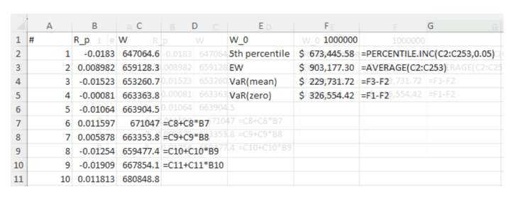
In Picture 2.1.1 the C column comprises the values of portfolio altering on account of fluctuations in portfolio returns. Some pattern calculation formulation are given in column D. Initially, computations begin by $1,000,000 from under and finally ends up above within the second row on account of descending order of dates.
Under is the analogous python code.
Parametric VaR
Computation of VaR takes an easier kind if we all know the chance distribution of returns or no less than we assume that the distribution belongs to the parametric household corresponding to regular distribution. In such case, the VaR might be straight computed primarily based on the usual deviation and a multiplicative issue akin to a given confidence stage. Typically, R* is adverse.
For extra comfort, we will write it as -R*. Assuming it’s usually distributed, we will affiliate it with a typical usually distributed random variable computed as

the place μ and σ symbolize the anticipated worth and customary deviation or R* respectively. So, we have now

Basically, all integrals in (2.2.2) symbolize the same amount – the chance of the portfolio worth on the finish of the funding horizon ending up inside the vary of ( (-infty, W^*) ) is ( 1 – c ). This amount clearly coincides with the chance that the portfolio return will fall inside ( (-infty, -|R^*|) ). Having transformed ( R^* ) into ( z ) customary regular amount by (2.2.1), we clearly see that above talked about integrals yield the identical consequence as a typical usually distributed random variable falling inside the interval ( (-infty, -z) ).
From this we clearly see that from ( c ) we will compute ( z ) and respectively, we will get well ( R^* = -zsigma + mu ). Right here we assume that the parameters ( mu ) and ( sigma ) are expressed on an annual foundation. If we specific the time interval in ( Delta t ) in years, then VaR relative to the imply might be expressed as follows:

and VaR computed as an absolute greenback loss (i.e. relative to zero) is

Instance:
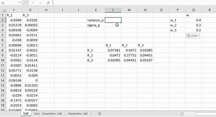
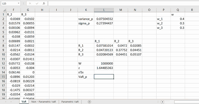
Suppose we have now yearly information of returns. 252 returns in {dollars} in whole. Allow us to take ( c = 95% ). So, the boldness stage is ( c = 95% ). First, we compute the portfolio values primarily based on returns by (2.1.1). Subsequent, the greenback returns are computed. The adverse greenback returns are considered losses. The imply and customary deviation of portfolio returns are computed first. ( z_{0.95} = 1.645 ). That is the usual regular quantile akin to 95% confidence stage. In different phrases, there’s 95% chance that the usual regular random variable takes the worth lower than this quantity: ( P(Z < z_{0.95}) = 95% ).
Subsequent, ( VaR(imply) = $450,598.39 ) and ( VaR(zero) = $474,751.86 ) are computed by (2.2.3) and (2.2.4) respectively. The connected Excel file comprises the computations.

Under is the analogous python code.
Portfolio VaR and predominant VaR instruments
Portfolio VaR
Portfolio VaR might be computed from the mixture of dangers related to underlying belongings. The portfolio fee of return is given by

the place N denotes the variety of belongings within the portfolio and Ri is the speed of return akin to the ith asset.
We are able to rewrite Rp in (3.1.1 a) by the vector notation:

Right here wT represents the transposed vector of weights and R is the vertical vector of charges of return of particular person belongings. We denote by μp the anticipated fee of return of the portfolio
and by σp2 we denote the portfolio variance

and by p2 we denote the portfolio variance

the place σij represents the covariance between ith and jth asset returns (i.e. between Ri and Rj). A extra handy manner of expressing σp2 by way of particular person asset variances and weights is in matrix kind

Denoting the covariance matrix as Σ, this will extra compactly be written by way of matrices as

The portfolio variance might be rewritten by way of greenback exposures x as

the place W denotes the preliminary portfolio worth. Assuming the person asset returns are usually distributed, the portfolio return itself, which is the linear mixture of collectively regular random variables, can also be usually distributed. So, if we outline by W the preliminary portfolio worth, the portfolio VaR turns into

the place z is the usual regular quantile akin to a sure confidence stage. e.g. P(Z < Z0.95) = 95%. On this case Z0.95 = 1.645.
Different frequent confidence ranges used are 90% and 99%. Corresponding z values are given under for handy reference:
| Confidence stage | z |
|---|---|
| 90% | 1.282 |
| 95% | 1.645 |
| 99% | 2.326 |
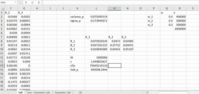
Instance:
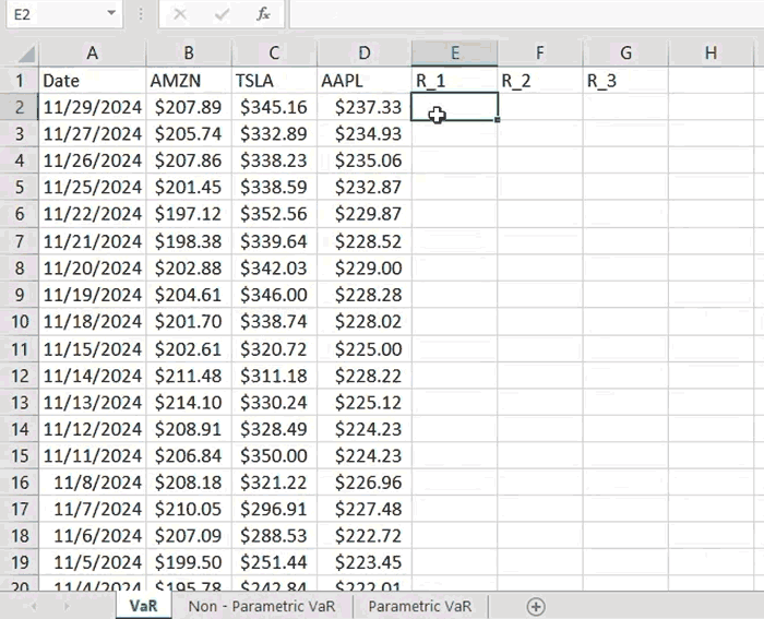
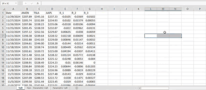
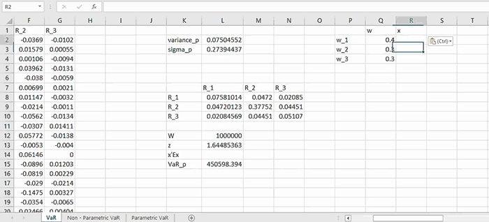
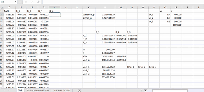
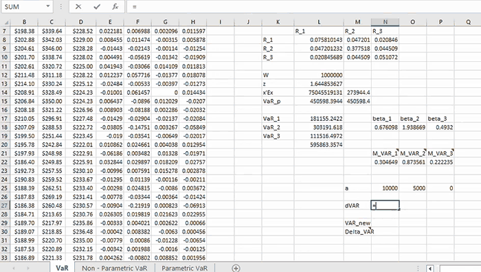
Given one-year month-to-month information of AMZN, TSLA and AAPL inside the time interval of 11/30/2023-11/29/2024, we compute the portfolio VaR and associated portions defined under. First, we compute the asset returns as

for every second t. The variance/covariance matrix for these asset returns is given under
=0.0758 0.0472 0.0209 0.0472 0.3775 0.0445 0.0209 0.0445 0.0511
Now contemplating the weights vector
w = [w1, w2, w3]T = [0.4, 0.3, 0.3]T
the estimated annualized variance of the portfolio returns is computed by (3.1.3 b) as follows
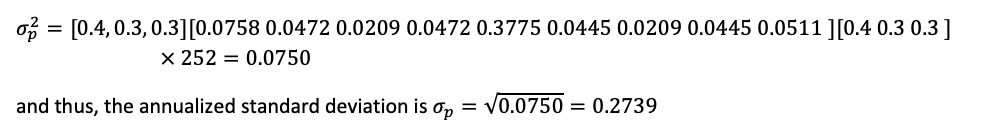
out of which we will straight compute the portfolio VaR assuming the preliminary portfolio worth W = $1,000,000 and the boldness stage of 95% (i.e. z = N-1(0.95) ≈ 1.64).

the portfolio VaR by (3.1.5) is

Alternatively, we might have first computed the portfolio customary deviation by way of greenback exposures after which compute VaR. First, we’d like the vector

and the variance of the portfolio by way of {dollars} by (3.1.4) is computed as proven under
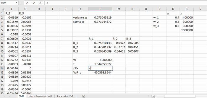
and correspondingly, the (full computation of) customary deviation is

and the portfolio VaR by (3.1.5) turns into

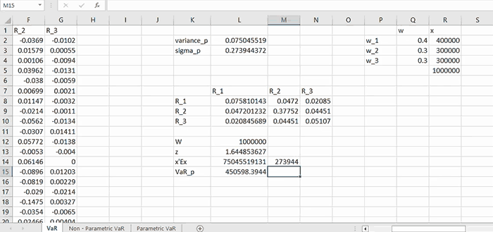
We interpret this amount as the biggest potential loss by 95% confidence stage, which might be incurred by the portfolio of $1,000,000 over a one-year horizon underneath regular circumstances. In less complicated phrases, there’s solely 5% chance that the precise loss incurred by the portfolio will surpass this quantity.
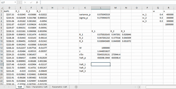
Particular person VaRs computed by the formulation (3.1.6) are
VaR1=$181,155.24
VaR2=$303,191.62
VaR3=$111,516.50
Notice that the sum of the person VaRs is $595,863.36 which is clearly not equal to the portfolio VaR. Portfolio VaR is much less because it takes benefit of the diversification impact.
Marginal VaR
VaR of an asset is a static amount which measures the uncertainty within the return of a given asset, taken in isolation. Nonetheless, when contemplating this asset as part of a portfolio, what issues is its contribution to the portfolio threat.
Allow us to start by an present portfolio consisting of N belongings. Now we contemplate including one unit of an asset i into the portfolio.
With the intention to measure the impression of this commerce on total portfolio threat, we use the software referred to as Marginal VaR.
First, we outline the spinoff of portfolio variance with respect to the ith asset weight as:

From which we derive

This amount measures the sensitivity of the portfolio threat with respect to a given asset weight. Changing this expression right into a VaR quantity yields the Marginal VaR for asset i

So long as beta of a given asset is outlined as

the connection between the Marginal VaR and the beta of a given asset might be expressed as follows

Instance cont’d:
Now we will compute the marginal VaRs for every asset inside the portfolio. First, we compute betas by (3.2.4)
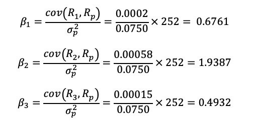
Correspondingly marginal VaRs are computed by (3.2.3 b)
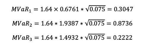
These portions are interpreted as a change in portfolio VaR on account of a further greenback publicity to a given asset. In different phrases, every extra $1 into the primary asset (AMZN) will enhance the portfolio VaR by $0.3047.
Incremental VaR
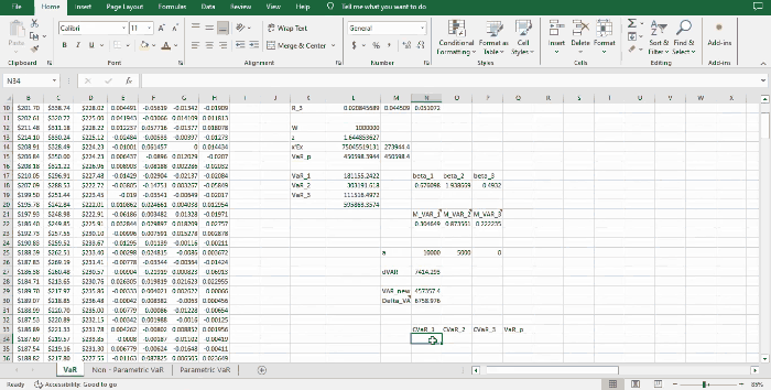
Suppose that we start with the preliminary portfolio VaRp. Then add new positions captured by the vector a. Components of this vector symbolize the modifications in every place. Consequently, we get hold of a brand new VaR and we denote it by VaRp+a. Thus the incremental VaR is outlined because the distinction between the brand new and previous VaRs as follows

From this formulation, it’s clear that calculation of an incremental VaR, i.e. the impact of a brand new place to the present portfolio VaR requires us to compute the VaR of the up to date portfolio in addition to the VaR of an present portfolio. Nonetheless, there’s a shortcut. Particularly, we will use the approximation approach. Increasing the VaRp+a across the authentic level VaRp yields

the place we ignore the remainder of the phrases assuming a is small enough. From which we have now

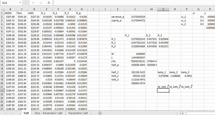
Instance Cont’d:
Allow us to start with the preliminary portfolio of $1 000 000 with positions vector x = [x1 x2 x3] = [400,000 300,000 300,000]. The VaR of such portfolio was computed in Instance 2.1 to be $450,598.39. Now contemplate a vector a = [10,000 5,000 0] of modifications in positions in every asset. i.e. we put a further $10,000 into AMZN, $5,000 into TSLA and we don’t change our place in AAPL. If we computed the VaR of the brand new portfolio by (3.1.5), that will turn out to be

So the incremental VaR computed exactly by (3.3.1 a) seems to be

Making use of the approximation approach (3.3.1 b), we’d get hold of

So the approximation yields nearly the identical consequence as exact methodology. The accuracy of approximation increased for smaller values in vector a.
Part VaR
With the intention to handle portfolio threat, it could be useful to have a threat decomposition of the present portfolio. This job shouldn’t be easy. The reason being that the portfolio volatility shouldn’t be a linear perform of its parts. Including up the person asset VaRs is not going to yield the portfolio VaR because it ignores the diversification impact. As a substitute, it could be actually helpful to have additive decomposition of VaR that acknowledges the ability of diversification.
In part 2.2 we lined marginal VaR stating that it measures the contribution of every asset to the present portfolio threat. Multiplying the marginal VaR by the present greenback place in asset offers a amount which we name the Part VaR of an asset i.

Roughly talking, the element VaR of the given asset i signifies how the portfolio VaR would change if the element (i.e. the given asset) was faraway from the portfolio. It must be famous that the standard of approximation improves when the VaR parts are small. Thus, the decomposition is extra correct for big portfolios having many small positions. Including up the Part VaRs of particular person belongings clearly yields the portfolio VaR, i.e.

right here the time period within the parenthesis is the beta of the portfolio with respect to itself which is unity.
Instance Cont’d:
The preliminary portfolio with $1 000 000 distributed into the positions x=400,000 300,000 300,000 had a VaR of $450,598.39. We are able to break up this quantity into the parts by (3.4.2)
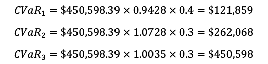
Not surprisingly, the sum of parts VaRs is the same as the overall portfolio VaR. In different phrases, the overall contribution of a given asset into the portfolio threat is the CVaR which corresponds to that asset. If we eliminated this asset from the portfolio, its threat would drop by the quantity of CVaR.
Consequently, we will conclude that VaR, when utilized appropriately offers a really helpful and intuitive measure of threat. It’s the largest potential loss {that a} portfolio could incur with a given confidence stage. There are numerous methods to compute VaR. If the distribution of portfolio return is unknown, a non-parametric strategy might be taken. In any other case, so long as the distribution of returns belongs to any parametric household, one can compute VaR in an easier manner.
As well as, there are helpful VaR instruments corresponding to Marginal VaR (MVaR), Incremental VaR (VaR) and Part VaR (CVaR) that are used to measure the results of a change in a given asset into the on your complete portfolio.
Particularly, Marginal VaR, outlined as a spinoff of a portfolio customary deviation with respect to a place taken in a sure asset, measures the impact of a single greenback change within the given asset on your complete portfolio threat.
Incremental VaR then again signifies by how a lot a given portfolio VaR would change on account of modifications within the positions.
Lastly, we described Part VaRs as instruments to decompose the overall portfolio VaR into the parts. It measures the contribution of a given asset into your complete portfolio threat.
Bibliography:
- Jorion, P. (2001). Worth At Threat: The brand new benchmark for managing Monetary threat. New York: McGraw Hill.
Additional Studying:Anticipated Shortfall (My different weblog – https://weblog.quantinsti.com/cvar-expected-shortfall/)
All investments and buying and selling within the inventory market contain threat. Any choice to position trades within the monetary markets, together with buying and selling in inventory or choices or different monetary devices is a private choice that ought to solely be made after thorough analysis, together with a private threat and monetary evaluation and the engagement {of professional} help to the extent you imagine crucial. The buying and selling methods or associated data talked about on this article is for informational functions solely.


